Using Time Series Analysis Electric Production by FB Prophet

I got the dataset from Kaggle for practicing time series analysis. 

https://www.kaggle.com/kandij/electric-production  

The data set used here has 2 columns, one column is the date and the other column relates to the consumption percentage. It includes the data from Dec 31,1984 to Dec 31,2017. For predicting the consumption of electricity in the coming future. 

I used time series analysis in Incorta notebooks using Facebook Prophet. 

	from pyspark.sql.functions import *
	from fbprophet import Prophet
	from sklearn.metrics import mean_squared_error
	from math import sqrt
	import pandas as pd
	from pyspark.sql.types import *
	import pickle
	import numpy as np
	#read data
	prod_demand_df = read("TimeSeries_ElectricProduction.ElectricProduction")
	#explore data
	prod_demand_df.printSchema()
	prod_demand_df.show(10)
	prod_demand_df.count()
	#I found the date is recognized as string
	#I tried to covert Date in string to a date for pandas
	prod_demand_df = prod_demand_df.withColumn('Date_date',to_date(prod_demand_df.DATE, 'MM-dd-yyyy')).drop(prod_demand_df.DATE)
	prod_demand_df.printSchema()
	prod_demand_df.show(10)
	#convert spark dataframe to pandas dataframe
	pdf = prod_demand_df.toPandas()
	# Check the format of 'Date' column
	pdf.info()
	#spark dataframe with the datatype still recognized as object
	# convert the 'Date' column to datetime format
	pdf['Date_date'] = pdf['Date_date'].astype('datetime64[ns]')
	# Check the format of 'Date' column
	pdf.info()
	#set index
	pdf.set_index(pd.DatetimeIndex(pdf['Date_date']))
	cutoff_date = "01-01-2017"
	before_cutoff = pdf["Date_date"] < cutoff_date
	after_cutoff = pdf["Date_date"] >= cutoff_date
	#filter data before date
	train = pdf.loc[before_cutoff]
	train.tail(10)
	train.info()
	print(type(train))
	#Rename the columns for Prophet
	#ds:date y:indicating the amount we want to predict
	train.columns = ['y','ds']
	#Create model
	prophet = Prophet(changepoint_prior_scale=0.15, daily_seasonality=False)
	prophet.fit(train)
	#Prediction
	future = list()
	for i in range(1, 13):
	date = '2017-%02d' % i
	print(i, date)
	future.append([date])
	future = pd.DataFrame(future)
	future.columns = ['ds']
	future['ds']= pd.to_datetime(future['ds'])
	future
	#Use the model(prophet) to make a forecast
	forecast=prophet.predict(future)
	forecast
	#filter data before date
	train = pdf.loc[before_cutoff]
	train
	#filter data after date
	test = pdf.loc[after_cutoff]
	test
	#concat dataframe
	pdf_with_forecast = pd.concat([train, test])
	pdf_with_forecast
	#yhat:predicted value
	test2 = forecast.loc[:,['ds', 'yhat']]
	test2
	#rename columns For the same column name, merge column
	test2.rename(columns = {'ds':'Date_date'}, inplace = True)
	test2
	#merge colume become 3 columes
	dtest = test.merge(test2, on="Date_date", how = 'inner')
	#Change the order of the columns
	dtest = dtest[['Date_date','Value','yhat']]
	dtest
	#import numpy as np
	train['yhat']=np.nan
	#Change the order of the columns
	dtrain = train[['Date_date','Value','yhat']]
	dtrain
	#concat two dataframes
	pdf_result = pd.concat([dtrain, dtest])
	pdf_result
	#covert pandas dataframe to spark dataframe
	result_df = spark.createDataFrame(pdf_result)
	save(result_df)

view raw Time Series Analysis Electric Production by Prophet hosted with ❤ by GitHub

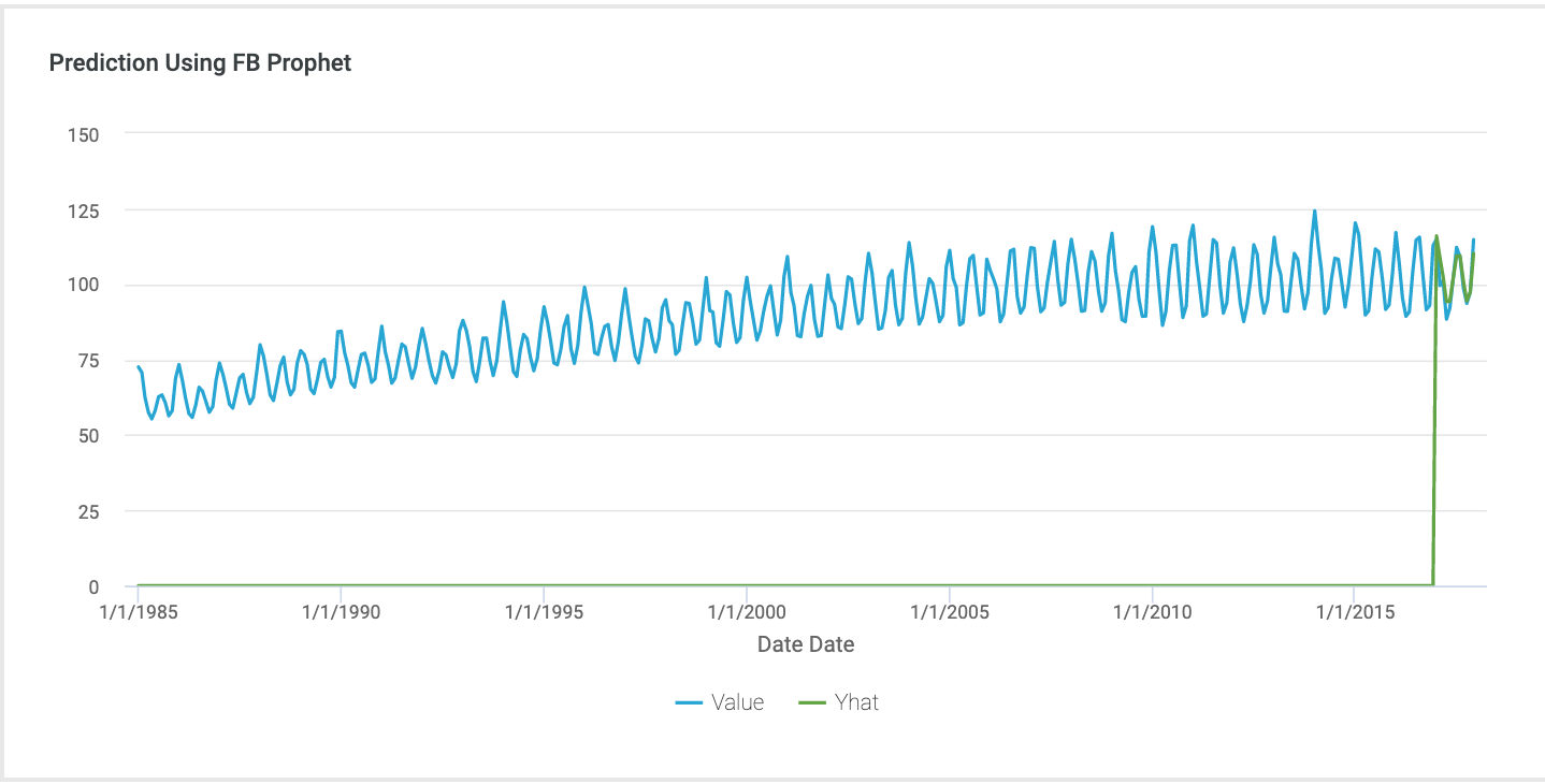
Here is the result in Incorta. The blue line showing original data, and the green line showing predict electric production.